Basic ROI analysis

This page will give instructions on how to use the fRAT to:

1. Create a voxel-wise tSNR map

2. Convert this voxel-wise map into an ROI based map

3. Understand the basics of the ROI analysis output

Note

This tutorial will focus on how to use the GUI version of the fRAT, as while many settings and functions can be accessed without the GUI, it is suggested that the GUI is used where possible until you already have familiarity with fRAT.

File setup

Tip

In the GUI, settings that will most often need changing are bold. Additionally, most settings have a tooltip giving an explanation of what the setting changes, and if relevant, how the format the setting expects.

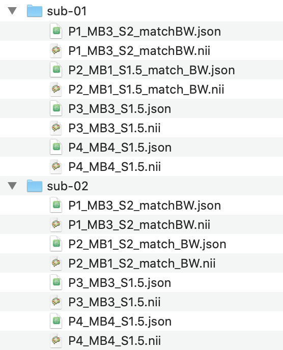
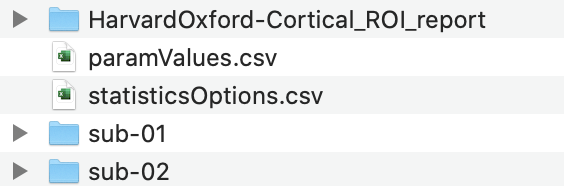
Before being able to run the ROI analysis, a few initial setup steps need to be taken. Firstly, the base folder should be structured with functional files organised into folders named using the format sub-{number} (e.g. sub-42):

Tip

Anatomical volumes can also be placed in this folder, however they should be moved from the func folder into the anat folder when it is created.

Next, enter the Parsing page found under the “Settings” panel in the GUI. The critical parameters setting indicates what the independent variables of the experiment are and will be used when labelling plots and creating the parameter csv file, whereas the critical parameters abbreviation setting indicates how these variables are represented in the filenames of the scans (if at all). For example, the critical parameters option may contain “Multiband, SENSE”, whereas the “critical parameters abbreviation” option will instead contain “mb, s”. In this case, the file name P1_MB3_S2_matchBW.nii will represent that Multiband 3 and SENSE 2 were used.

Note

The critical parameter settings are used to supply the names and file name abbreviations of the independent variables, therefore fRAT supports the use of any parameters (and any number of them).

If critical parameters is left blank, the ROI analysis will combine all datasets, regardless of the independent variable used for each file. This can be useful for calculating tSNR across the entire dataset, if the independent variable does not affect tSNR.

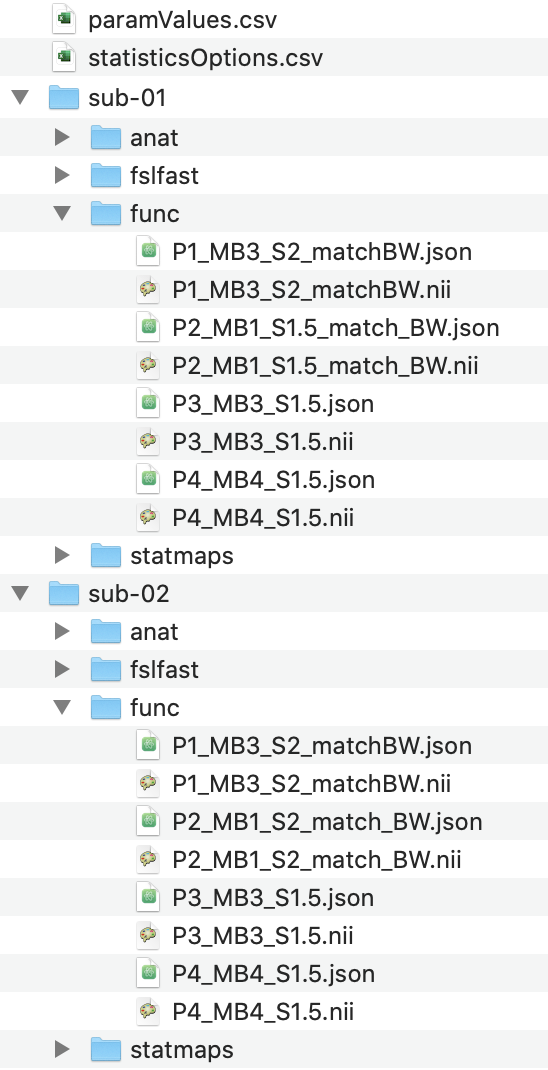
After filling these options in, select the “Make folder structure” option. This will create the basic folder structure required for the fRAT and will sort the files into the correct directory. After returning to the home page, click the Setup parameters button in the “Run” panel of the GUI. This will parse files names for critical parameters using the “critical parameters abbreviation” option set above, with the output being saved in paramValues.csv. This file should be checked before proceeding to make sure the correct parameters have been applied to each file. Another file, statisticsOptions.csv will by default also be created allowing you to set which post-hoc statistical tests to run. This file can be prevented from being created (for example, if the statistics step of the ROI analysis will not be used) by deselecting the “Automatically create statistics option file” option found in the Statistics menu. Alternatively, when running without the GUI, pass the –make_table flag when running fRAT.py, e.g. fRAT.py --make_table. After using the parsing GUI option, the necessary directories will be created with the files put into the folder func:

Warning

Make sure the lists of critical parameters given are in the same order, otherwise the critical parameter names will be applied to the wrong abbreviations.

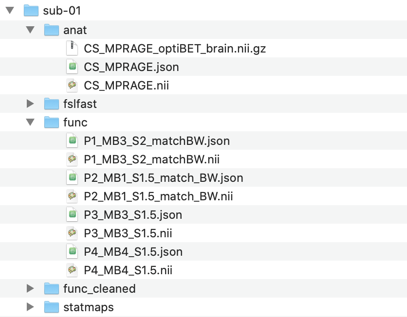
In the newly created anat folder, place a single skull stripped anatomical volume with the suffix “_brain”. The default BBR cost function for functional to anatomical registration requires a second, whole head, non-brain extracted volume to also be placed in the anat folder. This second file should not contain the word “brain” in the file name. While the BBR cost function also requires segmentation to have been ran using FAST, FAST will be automatically ran when running the analysis if this is not the case. However if you wish to run the segmentation ahead of time, the FAST output should be placed in the fslfast folder. If running the analysis on cortical regions (for example when using the Harvard-Oxford Cortical atlas), it is recommended that white matter and extracranial voxels are excluded from the analysis by setting the GUI option “Use FAST to only include grey matter” to true. While there is not currently support for using FAST to improve analysis of subcortical regions, support may be added in the future.

If FAST needs to be ran (either for BBR registration or to include only grey matter in the analysis) the accuracy of the skull stripped anatomical scans should still be assessed before running it. As overly conservative skull stripping can lead to skull being retained in the Resulting image, which FAST may then misidentify as grey matter. Conversely, overly liberal skull stripping can lead to parts of the brain being removed, meaning that these voxels will also not be included in any ROIs.

Note

To skull strip the anatomical files, it is highly recommended that optiBET is used as it has consistently produced the best brain extraction accuracy.

Voxel-wise tSNR map creation

Before creating the tSNR maps, click the Settings button in the “Statistical maps” section of the GUI. The default options will normally be sufficient, however if a noise scan has been added to the functional volumes, make sure under the “Image SNR calculation” header that information about this noise volume is given. This allows the fRAT to remove it when creating tSNR maps, and if creating iSNR maps, it will be used to calculate the noise value.

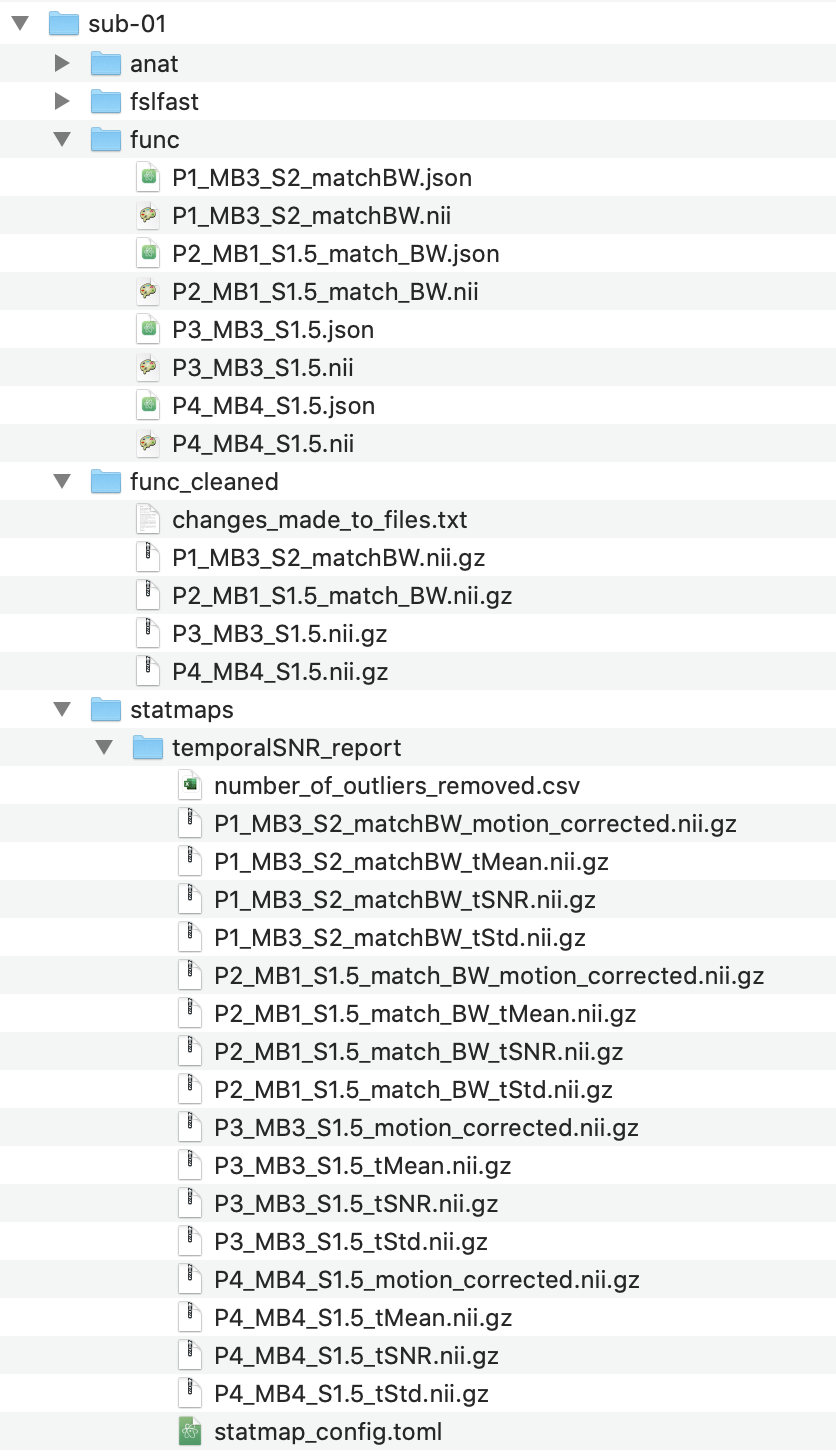
After inspecting the settings, to create the tSNR maps return to the home screen and in the “Run” panel of the “Statistical maps” section, select “Temporal SNR” from the dropdown menu then click “Make maps”. A file explorer will appear allowing you to navigate to the base folder where your subject folders are located. After selecting this base folder, tSNR maps for each functional volume will be calculated and placed into the statmaps folder. During creation of the maps, the folder func_preprocessed will be created, which contains functional volumes better suited to be used for the ROI analysis.

Note

The changes_made_to_files.txt contain details of how the files have been preprocessed. While func_preprocessed is the default folder that the ROI analysis will search for functional volumes in. This option can be changed using the Input folder name setting on the analysis screen of the GUI.

Running the ROI analysis

The same process for creating voxel-wise maps applies here, check each options menu from the “Settings” panel in the fRAT section of the GUI and then click the Run fRAT button to run the ROI analysis when you are ready to run the analysis. Again, the default options should be sufficient, however the bolded options are the ones most likely to need changing. In particular, the General option menu allows ROI analysis pipeline steps to be skipped if desired. Further, the “Statistical map folder” setting in the “Analysis” option menu should be changed to “temporalSNR_report”. If you wish to analyse any of the other files output by the tSNR map creation, the “Statistical map suffix” option can for example be changed to “tStd.nii.gz”.

The Atlas information section on the home page allows you to view the ROIs defined by each atlas, allowing you to select the most appropriate atlas to use for your analysis. To change which atlas is used for your analysis, change the Atlas option on the Analysis page. The numeric key corresponding to ROIs can be used in the ROIs to calculate statistics for and ROIs to plot settings (in the Statistics and Plotting menus respectively) to be more selective in ROI choice for statistics and figure creation. For example, for these settings, input 1,5,32 to specify ROIs 1, 5, and 32 for the chosen atlas or all for all ROIs.

Note

If running the Plotting or Statistics steps separately, the folder output by the analysis should be selected instead of the base folder.

Exploring ROI analysis output

After running the analysis, in addition to the folders created before, the base folder will now contain the newly created output folder:

Here is the folder structure of the output folder:

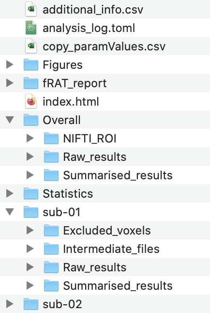
In the folder structure above:

• additional_info.csv contains further information about files such as the displacement values as measured during motion correction.

• analysis_log.toml is the configuration files used to run the analysis step (logs are also output for the statistics and plotting steps)

• copy_paramValues.csv is the parameter values used for the analysis.

• index.html is used to open the html report output by the plotting step.

• Statistics contains the statistical analysis output.

• Figures contains folders for each plot type created.

• fRAT_report contains the pages of the html report.

• Overall contains the final results, summarised across participants/sessions.

• sub-{number} contains the results computed for each participant.

In the Overall folder, Summarised_results will contain Participant_averaged_results and Session_averaged_results, with each folder containing a separate file for each parameter combination and also a combined_results.json file which combines the data from every other file in this folder. Participant averaged data first averages data within participants before being averaging between participants. Whereas session averaged results instead averages data between all sessions, disregarding which participant was scanned in each session; this can be useful where the statistical map being converted should be participant agnostic.

The NIFTI_ROI folder also found in the Overall folder contains the results from the the Participant_averaged_results and Session_averaged_results folders in .nii.gz format, with a separate file created for each statistic type and parameter combination. These are used for the brain grid figures during the plotting step. There are 3 types of NIFTI_ROI files:

• Standard (no suffix)

• Within ROI scaled

• Between ROI scaled

The “standard” files contain the actual statistic values for each ROI. “Within ROI scaled” and “between ROI scaled” files scale the values to a range between 0 and 100, with “Within ROI scaled” files have scaled each ROI based on the maximum value seen within that ROI across all parameters, and “between ROI scaled” files have scaled each ROI based on the maximum value seen across all ROIs across all parameters.

Warning

The plotting step uses the files found in the NIFTI_ROI folder to produce brain grids, however as scaling of these files is based on the other files and takes place during the analysis step, files present in this folder should not be deleted.

Raw_results, found in both the Overall and the sub-{number} folders contains the value of every voxel in each ROI. This data is used to produce histograms in the plotting step.

The Summarised_results folder in each sub-{number} folder, contains in addition to the results from each session for this participant, an Averaged_results folder. This folder has computed the mean average for every statistic across all sessions. This allows you to check if any of the participant results are outliers. In each sub-{number} folder there are also Intermediate_files and Excluded_voxels folders. The Intermediate_files folder contains all intermediate files produced by the fRAT, and can be used to produce figures or check the accuracy of the different preprocessing steps of the fRAT.

The Excluded_voxels contains 5 types of files, the first being the original fMRI volume (named handily fMRI_volume). This is placed here to more easily create figures using fsleyes. The next type of file is the pre-corrected standard to native space registered ROI atlas (named orig_mni_to_{fMRI_volume_name}). Next is the files which show each stage of corrections made to the ROI atlas file. Each of these files is named in the format: ExcludedVoxStage{stage}_{fMRI_volume_name}_{method}. For example: ExcludedVoxStage3_P2_MB1_S2_match_BW_noiseThreshOutliers. Next is the binary mask files, the first named binary_mask_{fMRI_volume_name} is merely a binarised mask of voxels retained after the above correction stages. The next binary mask file named binary_mask_filled_{fMRI_volume_name} is the binary mask with holes filled using the fslmaths flag -fillh. The last binary mask file (filled_voxels_{fMRI_volume_name}) highlights which voxels were filled in during the previous step. Finally, is the ROI atlas which has undergone correction and filled in gaps in its mask. This is the final ROI atlas used for the analysis and is named final_mni_to_{fMRI_volume_name}.

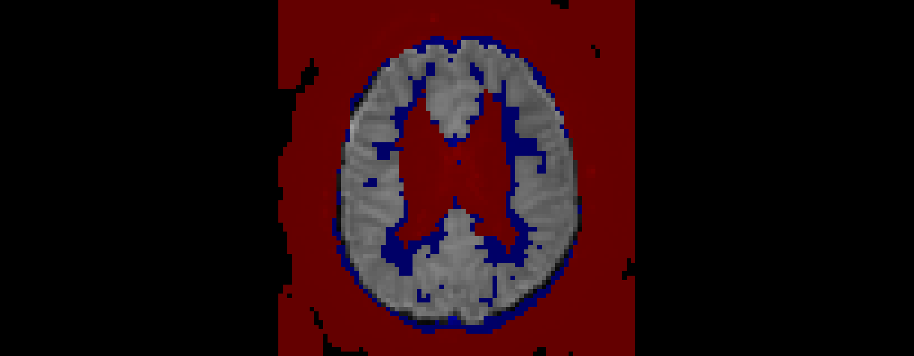
A visualisation of which voxels have been retained after correction. Red voxels were excluded during the original standard to native space registration, whereas blue voxels have been excluded as they have been marked as potentially white matter. This visualisation was created by overlaying each stage of the excluded voxel files on top of the original functional volume.

The final standard to native space registered ROI atlas overlaid on the original functional volume.

Both the print results and interactive table GUI options can be used to explore the data once the analysis has been ran. The print results option prints the results for the selected region of interests to the terminal, whereas the interactive table option opens up the results in a browser window.